ARTICLE BY MR. EZRA SALAMAT
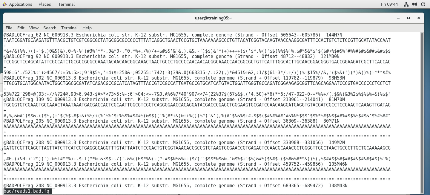
The previous three chapters discussed the wet-lab workflow of DNA sequencing. Upon completion of the actual sequencing process, sequencing platforms like the Illumina MiSeq can produce an output of up to 15Gb worth of data, amounting to up to 25 million reads. One might think that the immediate output of such sequencing process would be a whole genome sequence such as this:  ...when in fact the actual output actually looks more of something like this instead: 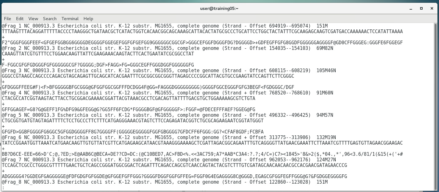 Now the actual output doesn't look anything remotely useful at all... and in fact it isn't... at least in its current form. The Illumina platform outputs the individual sequences of all several millions worth of reads, each only 150-300bp long (depending on the kit used). These sequences need to be processed into a form usable for scientist... and that's where bioinformatics tools come in. If you remember in Chapter 2, we mentioned that the Illumina sequencing platform can only sequence short stretches of DNA. So instead of sequencing the entire length of the genome from one end to another, one base at a time, Illumina reads millions of smaller fragments in parallel, which can then be assembled later. 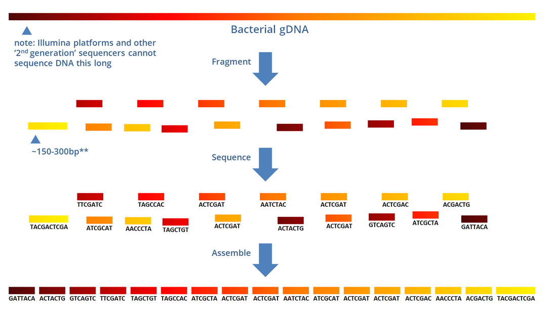 OVERVIEW OF QUALITY SCORESThe Illumina platform outputs its data in FastQ Format (sample shown below). Each read (red box) starts with an @ symbol, and is composed of four lines (parts):
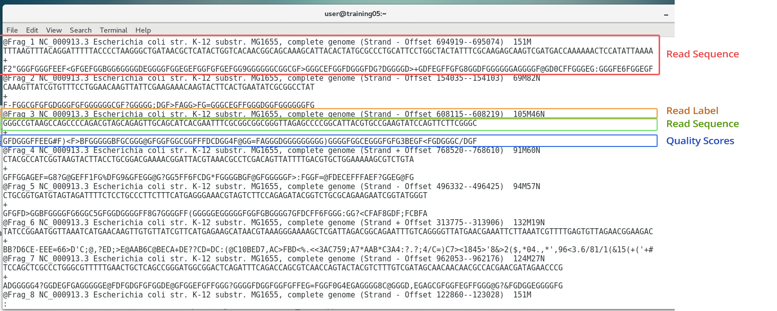 Image: FastQ File As you can see in the image above, the Quality Scores are encoded in single characters (a number, letter, or symbol), each representing a quality score based on the ASCII table. The Illumina ASCII-Quality Score code table is shown below:  Image from: https://support.illumina.com/help/BaseSpace_OLH_009008/Content/Source/Informatics/BS/QualityScoreEncoding_swBS.htm Here, a symbol corresponds to a Q-score, which is a compact expression of error probability. For instance, the symbol "?" has a corresponding Q-score of 30. We can then determine the error probability using the formula: Q(A) =-10 log10(P(~A)) where: Q(A), expresses the probability that A is not true P(~A) is the estimated probability of an assertion A being wrong. We can also use pre-computed tables, such as the one below:  Based on the table above, a Q-score of 30 has an Error Probability of 0.001- that is, the probability of an incorrect base call is 1 in 1,000 (or 0.1%). Let's look at an actual example below: 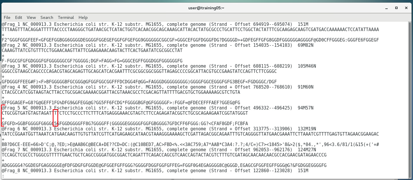 In the FastQ file above, the boxed nucleotide sequence "T" has a quality symbol of "5". Looking back at the tables above, "5" corresponds to a Quality score of 20, which means that it has an error probability of 0.01 (1%). This means that for that position, the machine is 99% sure that the nucleotide is a "T". SEQUENCE QUALITY CONTROLConverting raw reads to an assembled genome requires a pipeline - or series of processes that filters, sorts, and assembles the reads. The first step is to separate the good reads from the bad ones, based on the overall quality score of each read. A threshold is set, and all reads above a certain threshold (e.g. 10% error rate) are discarded. A dedicated bioinformatics program called "AfterQC" is used to sort the good and bad reads. Below is an example of a FastQ file sorted into good and bad reads. In the images below, 1,034,328 reads were sorted into 509,328 good reads and 525,000 bad reads.
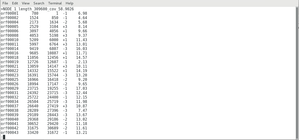
 SEQUENCE ASSEMBLY (SIMPLIFIED OVERVIEW)Only the good reads will be used in the next step, which is the assembly step. There are several programs available, each using its own algorithms (i.e. set of mathematical processes/formula), but we will look into a program called SPAdes (St. Petersburg genome assembler) , shown below: 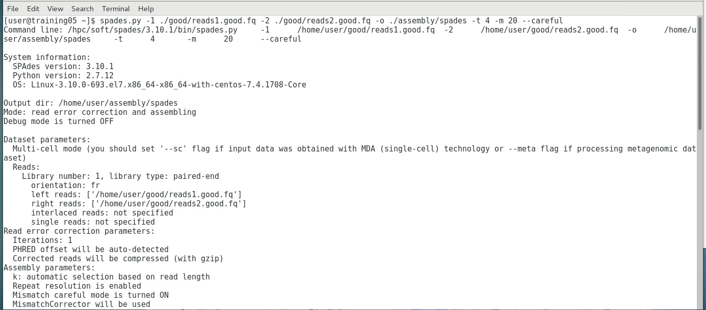 Image: Initialization page of SPAdes. Like most Bioinformatics programs, SPAdes lack a dedicated UI (User Interface) and runs using command lines. SPAdes aligns the reads and determines the most likely arrangement in which they are interconnected, using a complex algorithm (i.e. it employs multisized de Bruijn graph). You can learn more about SPAdes at the Center for Algorithmic Biotechnology webpage.  Image: SPAdes output files (left), and QUAST-generated SPAdes report (right) SPAdes generates longer sequences called contigs, scaffolds,and assemblies by joining reads together - visible as fasta files above. A report above (generated by the QUAST tool) indicates that there were four >50,000 bp contigs successfully, eight >25000 bp contigs successfully assembled, and so on.  Image: Simplified diagram of Genome Assembly The image above shows a simplified diagram of how the assembly was done. Short contigs are assembled into longer scaffolds, which are then assembled further into assemblies. In most cases, the initial assemblies may correspond to a considerable portion of the whole genome sequence (e.g. 98% of the whole genome), but it may still contain gaps (as shown above) that may need to be resolved by another sequencing method (such as capillary sequencing. Once the gaps has been sequenced, the gap sequence is aligned to the initial assembly, resulting to the final assembly (i.e. whole genome; sample shown below). 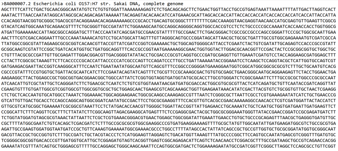 Image: portion of an E. coli genome sequence The Image below shows how all the 500,000+ good reads (multicolored dots) reads map into the final assembly, which shows the immense amount of computational power needed to perform such a large scale assembly of short read sequences.  Image: Read Map generated by TABLET: a graphical viewer for next generation sequence assemblies and alignments
|